6 minutes
Maglev - A Next-Generation Load Balancer
When reading Google’s SRE book, I came across the section on load balancing. The book breaks up load balancing into three levels:
- DNS level
- Network level/Virtual IP level
- Datacenter level
While I was familiar with the Datacenter level (aka reverse proxy load balancing) and DNS load balancing (achieved partially through round robin DNS), I had never looked at network-level load balancing. After reading this section, I was fascinated with how their network-level load balancing works.
After some research online, I realized that the system they were referring to was their load balancer called Maglev. In 2016, Google released a paper detailing Maglev and how they built it. If you’re interested in the nitty-gritty details, you can read the paper here. It’s a dense but fascinating read. I could spend a huge amount of time going into all the details of what makes Maglev interesting, but instead, I’ll focus on two aspects: Maglev hashing and packet encapsulation.
Introduction
Before anything else, I’ll describe the function of a network load balancer. The job of a network load balancer is to distribute packets destined for a “virtual IP address” to a set of backends evenly. Take the following picture as an example:
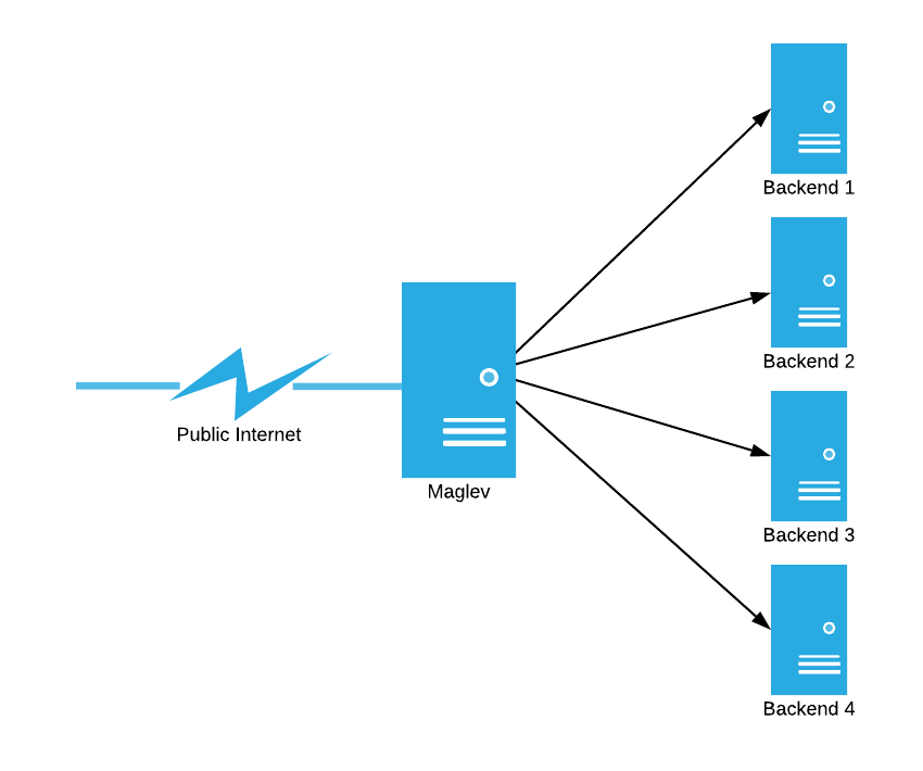
In this example, the job of Maglev is to deliver all of the packets coming in from the public internet evenly to backends 1-4.
Maglev Hashing
The first part of load balancing is actually deciding which backend to send an incoming packet to. In network load balancing, we are just looking at the IP layer, so we can’t keep track of things like which backend has the most TCP connections open to it. Since we can’t keep track of current state, we have to figure out how to distribute packets evenly just based on some attribute of the packet. Assume we pick out some attribute of each packet (this is usually a hashed combination of source IP and source port) and call id id. Then, we can treat id as an integer and evenly distribute packets to backends using the function backend = id (mod n) where n is our number of backends. Assuming an even distribution of IDs, this method will evenly distribute packets to backends, and it will keep sending packets from the same source to the same backend.
So, is it that simple? It seems like we’ve achieved what we want to - even distribution - with no downsides. Consider what happens when our n increases or decreases by even 1, however. In this case, since we don’t know the range of our id hash function, which backend our packets go to could be completely changed for all connections. This would mean that all open client connections would be broken, which is certainly not desirable behavior. To see this in action, let’s look at the example of where to send incoming packets with 5 backends versus with 4 backends.
| id | id (mod 4) | id (mod 5) |
|---|---|---|
| 717 | 1 | 2 |
| 561 | 1 | 1 |
| 544 | 0 | 4 |
| 67 | 3 | 2 |
| 310 | 2 | 0 |
| 626 | 2 | 1 |
As you can see, all the packet flows are disrupted except that for the packet with id 561. Since we will certainly be adding and removing backends live, this is unacceptable behavior. This is where consistent hashing comes to the rescue. Consistent hashing is very complicated, but the short of it is that it provides a way for minimal disruption when adding and removing backends. With consistent hashing, instead of all the packet flows being disrupted, at most 1/n (where n is the number of the backends) of the packets flows are disrupted.
There are many trade-offs with different kinds of consistent hashing that this article explains better than I can, but in essence, there are three things you can optimize for in consistent hashing: memory usage, lookup speed, and hashtable rebuild speed. You can typically have 2 of these at once, but you can never have all 3 without making some other very significant tradeoff. Google’s solution, called Maglev Hashing, optimizes for the first two. It assumes node failures are uncommon, and in making that assumption, it can get low memory usage with high lookup speed and minimal disruption when new backends are added but poor rebuild speed when a backend fails. This is a pretty reasonable assumption, and it turns out to work extremely well in the context of network load balancing.
Now that we know how to pick backends, let’s actually talk about how we send data to backends.
Packet Encapsulation
First, let’s consider the reverse proxy method of load balancing. In this method, connections are taken in by the load balancer. The balancer then initiates a new connection to the appropriate backend for the connection, and proxies the connections together, allowing the client to indirectly talk to a backend. This method looks like this:
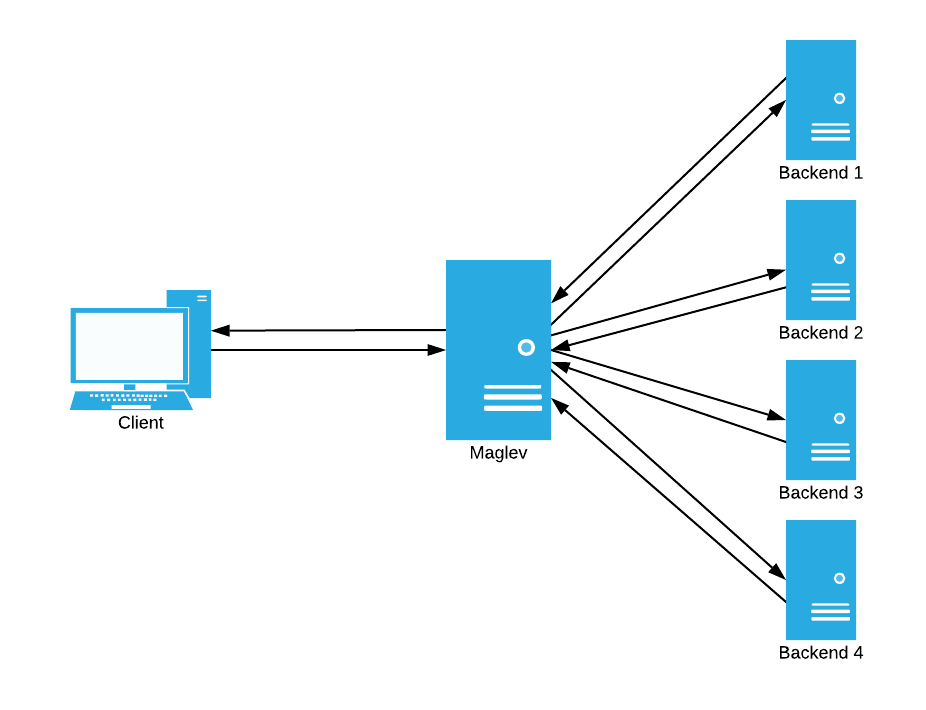
In this design, the load balancer has to do the following:
- Keep track of all active connections
- Proxy data between connections for all connections
- Pass both ingress and egress traffic for all the backends
While this is acceptable (and even desired) for a datacenter load balancer, we can’t pass packets at the scale a network load balancer needs to using this design. This is where packet encapsulation comes into play.
The solution that Google found to this problem was to use the following algorithm:
- Maglev hash the packet to determine its backend
- Wrap the packet in a layer of GRE (generic routing encapsulation)
- Send the encapsulated packet to the desired backend
- Have the backend break the packet of the encapsulation and fully process it
- Have the backend directly reply to this packet.
Did you catch that last step? Since we’re using encapsulation, the backend is seeing the original packet as received by the load balancer, so it can directly reply to the packet. We can see this in action on an example packet flow:
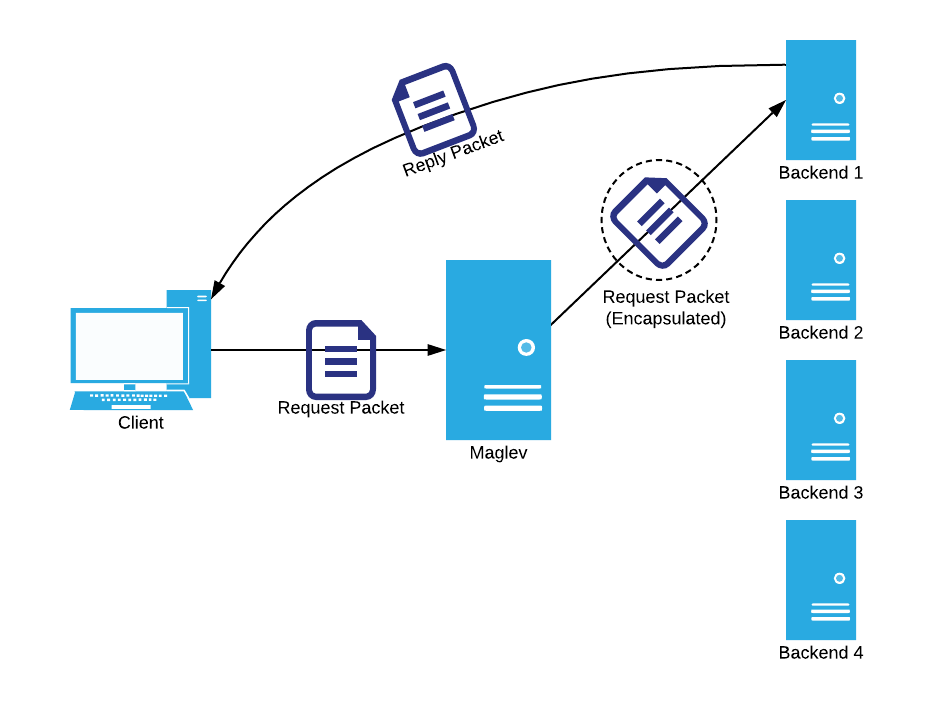
The fact that the backend can directly reply is a huge benefit of the encapsulation method. To see why, consider the use case of YouTube. When a user requests to see a video, the request payload is very small, only containing metadata about what video they want to watch. The reply, however, is gigantic since it’s a full video of up to 8K quality! With this method, the load balancer only only has to worry about the request, meaning it can handle drastically more traffic than a reverse proxy can.
Personally, I thought this was the most interesting part of Maglev. I had only ever thought to use GRE as a site-to-site VPN, but this gave me a whole new outlook on what it could do.
Conclusion
Maglev brings a ton of interesting concepts to the table and combines them in a way we’ve never really seen before. I could only cover two things here, but tech like ECMP and RPC also play a huge role in how Maglev works. If you’re interested, I highly encourage reading the paper.
Thanks for reading! Look below for a shameless plug.
Shameless Plug
As I said, I found Google’s ideas on network load balancers fascinating. In fact, I found it so interesting that I decided to implement it myself! If you’re interested in seeing how some of these ideas are implemented, I’m writing my own version of Maglev called Caplance here. At the time of writing this, I’m working on setting up automated testing with Mininet, and I’ll probably write more in the coming weeks as I make more progress on the load balancer.